DEMetropolis and DEMetropolis(Z) Algorithm Comparisons

import time

import arviz as az
import matplotlib.pyplot as plt
import numpy as np
import pandas as pd
import pymc as pm
import scipy.stats as st

print(f"Running on PyMC v{pm.__version__}")

WARNING (pytensor.tensor.blas): Using NumPy C-API based implementation for BLAS functions.

Running on PyMC v0+untagged.9358.g8ea092d

az.style.use("arviz-darkgrid")
rng = np.random.default_rng(1234)

Background

For continuous variables, the default PyMC sampler (NUTS) requires that gradients are computed, which PyMC does through autodifferentiation. However, in some cases, a PyMC model may not be supplied with gradients (for example, by evaluating a numerical model outside of PyMC) and an alternative sampler is necessary. Differential evolution (DE) Metropolis samplers are an efficient choice for gradient-free inference. This notebook compares the DEMetropolis and the DEMetropolisZ samplers in PyMC to help determine which is a better option for a given problem.

The samplers are based on and ter Braak and Vrugt [2008] and are described in the notebook DEMetropolis(Z) Sampler Tuning. The idea behind differential evolution is to use randomly selected draws from other chains (DEMetropolis), or from past draws of the current chain (DEMetropolis(Z)), to make more educated proposals, thus improving sampling efficiency over the standard Metropolis implementation. Note that the PyMC implementation of DEMetropolisZ is slightly different than in ter Braak and Vrugt [2008], namely, each DEMetropolisZ chain only looks into its own history, whereas the ter Braak and Vrugt [2008] algorithm has some mixing across chains.

In this notebook, 10 and 50-dimensional multivariate normal target densities will be sampled with both DEMetropolis and DEMetropolisZ samplers. Samplers will be evaluated based on effective sample size, sampling time and MCMC chain correlation \((\hat{R})\). Samplers will also be compared to NUTS for benchmarking. Finally, MCMC traces will be compared to the analytically calculated target probability densities to assess potential bias in high dimensions.

Key Take-Aways (TL;DR)

Based on the results in this notebook, use DEMetropolisZ for lower dimensional problems (\(\approx10D\)), and DEMetropolis for higher dimensional problems (\(\approx50D\))

• The DEMetropolisZ sampler was more efficient (ESS per second sampling) than DEMetropolis.

• The DEMetropolisZ sampler had better chain convergence \((\hat{R})\) than DEMetropolis.

• Bias was evident in the DEMetropolisZ sampler at 50 dimensions, resulting in reduced variance compared to the target distribution. DEMetropolis more accurately sampled the high dimensional target distribution, using \(2D\) chains (twice the number of model parameters).

• As expected, NUTS was more efficient and accurate than either Metropolis-based algorithms.

Helper Functions

This section defines helper functions that will be used throughout the notebook.

D-dimensional MvNormal Target Distribution and PyMC Model

gen_mvnormal_params generates the parameters for the target distribution, which is a multivariate normal distribution with \(\sigma^2\) = [1, 2, 3, 4, 5] in the first five dimensions and some correlation thrown in.

Show code cell source

Hide code cell source

def gen_mvnormal_params(D):
    # means=zero
    mu = np.zeros(D)
    # sigma**2 = 1 to start
    cov = np.eye(D)
    # manually adjust the first 5 dimensions
    # sigma**2 in the first 5 dimensions = 1, 2, 3, 4, 5
    # with a little covariance added
    cov[:5, :5] = np.array(
        [
            [1, 0.5, 0, 0, 0],
            [0.5, 2, 2, 0, 0],
            [0, 2, 3, 0, 0],
            [0, 0, 0, 4, 4],
            [0, 0, 0, 4, 5],
        ]
    )
    return mu, cov

make_model accepts the multivariate normal parameters mu and cov and outputs a PyMC model.

Show code cell source

Hide code cell source

def make_model(mu, cov):
    with pm.Model() as model:
        x = pm.MvNormal("x", mu=mu, cov=cov, shape=(len(mu),))
    return model

Sampling

sample_model performs MCMC, returns the trace and the sampling duration.

Show code cell source

Hide code cell source

def sample_model(
    model, D, run=0, step_class=pm.DEMetropolis, cores=1, chains=1, step_kwargs={}, sample_kwargs={}
):
    # sampler name
    sampler = step_class.name
    # sample model

    # if nuts then do not provide step method
    if sampler == "nuts":
        with model:
            step = step_class(**step_kwargs)
            t_start = time.time()
            idata = pm.sample(
                # step=step,
                chains=chains,
                cores=cores,
                initvals={"x": [0] * D},
                discard_tuned_samples=False,
                progressbar=False,
                random_seed=2020 + run,
                **sample_kwargs
            )
            t = time.time() - t_start

    # signature for DEMetropolis samplers
    else:
        with model:
            step = step_class(**step_kwargs)
            t_start = time.time()
            idata = pm.sample(
                step=step,
                chains=chains,
                cores=cores,
                initvals={"x": [0] * D},
                discard_tuned_samples=False,
                progressbar=False,
                random_seed=2020 + run,
                **sample_kwargs
            )
            t = time.time() - t_start

    return idata, t

calc_mean_ess calculates the mean ess for the dimensions of the distribution.

Show code cell source

Hide code cell source

def calc_mean_ess(idata):
    return az.ess(idata).x.values.mean()

calc_mean_rhat calculates the mean \(\hat{R}\) for the dimensions of the distribution.

Show code cell source

Hide code cell source

def calc_mean_rhat(idata):
    return az.rhat(idata).x.values.mean()

sample_model_calc_metrics wraps the previously defined functions: samples the model, calculates the metrics and packages the results in a Pandas DataFrame

Show code cell source

Hide code cell source

def sample_model_calc_metrics(
    sampler,
    D,
    tune,
    draws,
    cores=1,
    chains=1,
    run=0,
    step_kwargs=dict(proposal_dist=pm.NormalProposal, tune="scaling"),
    sample_kwargs={},
):
    mu, cov = gen_mvnormal_params(D)
    model = make_model(mu, cov)
    idata, t = sample_model(
        model,
        D,
        step_class=sampler,
        cores=cores,
        chains=chains,
        run=run,
        step_kwargs=step_kwargs,
        sample_kwargs=dict(sample_kwargs, **dict(tune=tune, draws=draws)),
    )
    ess = calc_mean_ess(idata)
    rhat = calc_mean_rhat(idata)
    results = dict(
        Sampler=sampler.__name__,
        D=D,
        Chains=chains,
        Cores=cores,
        tune=tune,
        draws=draws,
        ESS=ess,
        Time_sec=t,
        ESSperSec=ess / t,
        rhat=rhat,
        Trace=[idata],
    )
    return pd.DataFrame(results)

concat_results concatenates the results and does a some data wrangling and calculating.

Show code cell source

Hide code cell source

def concat_results(results):
    results_df = pd.concat(results)

    results_df["Run"] = results_df.Sampler + "\nChains=" + results_df.Chains.astype(str)

    results_df["ESS_pct"] = results_df.ESS * 100 / (results_df.Chains * results_df.draws)
    return results_df

Plotting

plot_comparison_bars plots the ESS and \(\hat{R}\) results for comparison.

Show code cell source

Hide code cell source

def plot_comparison_bars(results_df):
    fig, axes = plt.subplots(1, 3, figsize=(10, 5))
    ax = axes[0]
    results_df.plot.bar(y="ESSperSec", x="Run", ax=ax, legend=False)
    ax.set_title("ESS per Second")
    ax.set_xlabel("")
    labels = ax.get_xticklabels()

    ax = axes[1]
    results_df.plot.bar(y="ESS_pct", x="Run", ax=ax, legend=False)
    ax.set_title("ESS Percentage")
    ax.set_xlabel("")
    labels = ax.get_xticklabels()

    ax = axes[2]
    results_df.plot.bar(y="rhat", x="Run", ax=ax, legend=False)
    ax.set_title(r"$\hat{R}$")
    ax.set_xlabel("")
    ax.set_ylim(1)
    labels = ax.get_xticklabels()

    plt.suptitle(f"Comparison of Runs for {D} Dimensional Target Distribution", fontsize=16)
    plt.tight_layout()

plot_forest_compare_analytical plots the MCMC results for the first 5 dimensions and compares to the analytically calculated probability density.

Show code cell source

Hide code cell source

def plot_forest_compare_analytical(results_df):
    # extract the first 5 dimensions
    summaries = []
    truncated_traces = []
    dimensions = 5
    for row in results_df.index:
        truncated_trace = results_df.Trace.loc[row].posterior.x[:, :, :dimensions]
        truncated_traces.append(truncated_trace)
        summary = az.summary(truncated_trace)
        summary["Run"] = results_df.at[row, "Run"]
        summaries.append(summary)
    summaries = pd.concat(summaries)

    # plot forest
    axes = az.plot_forest(
        truncated_traces, combined=True, figsize=(8, 3), model_names=results_df.Run
    )
    ax = axes[0]

    # plot analytical solution
    yticklabels = ax.get_yticklabels()
    yticklocs = [tick.__dict__["_y"] for tick in yticklabels]
    min, max = axes[0].get_ylim()
    width = (max - min) / 6
    mins = [ytickloc - (width / 2) for ytickloc in yticklocs]
    maxes = [ytickloc + (width / 2) for ytickloc in yticklocs]
    sigmas = [np.sqrt(sigma2) for sigma2 in range(1, 6)]
    for i, (sigma, min, max) in enumerate(zip(sigmas, mins[::-1], maxes[::-1])):
        # scipy.stats.norm to calculate analytical marginal distribution
        dist = st.norm(0, sigma)
        ax.vlines(dist.ppf(0.03), min, max, color="black", linestyle=":")
        ax.vlines(dist.ppf(0.97), min, max, color="black", linestyle=":")
        ax.vlines(dist.ppf(0.25), min, max, color="black", linestyle=":")
        ax.vlines(dist.ppf(0.75), min, max, color="black", linestyle=":")
        if i == 0:
            ax.text(dist.ppf(0.97) + 0.2, min, "Analytical Solutions\n(Dotted)", fontsize=8)

    # legend
    labels = ax.get_legend().__dict__["texts"]
    labels = [label.__dict__["_text"] for label in labels]
    handles = ax.get_legend().__dict__["legendHandles"]
    ax.legend(
        handles[::-1],
        labels[::-1],
        loc="center left",
        bbox_to_anchor=(1, 0.5),
        fontsize="medium",
        fancybox=True,
        title="94% and 50% HDI",
    )
    ax.set_title(
        f"Comparison of MCMC Samples and Analytical Solutions\nFirst 5 Dimensions of {D} Dimensional Target Distribution"
    )

plot_forest_compare_analytical_dim5 plots the MCMC results for the fift 5 dimension and compares to the analytically calculated probability density for repeated runs for the bias check.

Show code cell source

Hide code cell source

def plot_forest_compare_analytical_dim5(results_df):
    # extract the 5th dimension
    summaries = []
    truncated_traces = []
    dimension_idx = 4
    for row in results_df.index:
        truncated_trace = results_df.Trace.loc[row].posterior.x[:, :, dimension_idx]
        truncated_traces.append(truncated_trace)
        summary = az.summary(truncated_trace)
        summary["Sampler"] = results_df.at[row, "Sampler"]
        summaries.append(summary)
    summaries = pd.concat(summaries)
    cols = ["Sampler", "mean", "sd", "hdi_3%", "hdi_97%", "ess_bulk", "ess_tail", "r_hat"]
    summary_means = summaries[cols].groupby("Sampler").mean()

    # scipy.stats.norm to calculate analytical marginal distribution
    dist = st.norm(0, np.sqrt(5))
    summary_means.at["Analytical", "mean"] = 0
    summary_means.at["Analytical", "sd"] = np.sqrt(5)
    summary_means.at["Analytical", "hdi_3%"] = dist.ppf(0.03)
    summary_means.at["Analytical", "hdi_97%"] = dist.ppf(0.97)

    # plot forest
    colors = plt.rcParams["axes.prop_cycle"].by_key()["color"]
    axes = az.plot_forest(
        truncated_traces,
        combined=True,
        figsize=(8, 3),
        colors=[colors[0]] * reps + [colors[1]] * reps + [colors[2]] * reps,
        model_names=results_df.Sampler,
    )
    ax = axes[0]

    # legend
    labels = ax.get_legend().__dict__["texts"]
    labels = [label.__dict__["_text"] for label in labels]
    handles = ax.get_legend().__dict__["legendHandles"]
    labels = [labels[reps - 1]] + [labels[reps * 2 - 1]] + [labels[reps * 3 - 1]]
    handles = [handles[reps - 1]] + [handles[reps * 2 - 1]] + [handles[reps * 3 - 1]]
    ax.legend(
        handles[::-1],
        labels[::-1],
        loc="center left",
        bbox_to_anchor=(1, 0.5),
        fontsize="medium",
        fancybox=True,
        title="94% and 50% HDI",
    )
    ax.set_title(
        f"Comparison of MCMC Samples and Analytical Solutions\n5th Dimension of {D} Dimensional Target Distribution"
    )

    # plot analytical solution as vlines
    ax.axvline(dist.ppf(0.03), color="black", linestyle=":")
    ax.axvline(dist.ppf(0.97), color="black", linestyle=":")
    ax.text(dist.ppf(0.97) + 0.1, 0, "Analytical Solution\n(Dotted)", fontsize=8)
    return summaries, summary_means

Experiment #1. 10-Dimensional Target Distribution

All traces are sampled with cores=1. Surprisingly, sampling was slower using multiple cores rather than one core for both samplers for the same number of total samples.

DEMetropolisZ and NUTS are sampled with four chains, and DEMetropolis are sampled with more based on ter Braak and Vrugt [2008]. DEMetropolis requires that, at a minimum, \(N\) chains are larger than \(D\) dimensions. However, {cite:t}terBraak2008differential recommends that \(2D<N<3D\) for \(D<50\), and \(10D<N<20D\) for higher dimensional problems or complicated posteriors.

The following code lays out the runs for this experiment.

# dimensions
D = 10
# total samples are constant for Metropolis algorithms
total_samples = 200000
samplers = [pm.DEMetropolisZ] + [pm.DEMetropolis] * 3 + [pm.NUTS]
coreses = [1] * 5
chainses = [4, 1 * D, 2 * D, 3 * D, 4]
# calculate the number of tunes and draws for each run
tunes = drawses = [int(total_samples / chains) for chains in chainses]
# manually adjust NUTs, which needs fewer samples
tunes[-1] = drawses[-1] = 2000
# put it in a dataframe for display and QA/QC
pd.DataFrame(
    dict(
        sampler=[s.name for s in samplers],
        tune=tunes,
        draws=drawses,
        chains=chainses,
        cores=coreses,
    )
).style.set_caption("MCMC Runs for 10-Dimensional Experiment")

MCMC Runs for 10-Dimensional Experiment

	sampler	tune	draws	chains	cores
0	DEMetropolisZ	50000	50000	4	1
1	DEMetropolis	20000	20000	10	1
2	DEMetropolis	10000	10000	20	1
3	DEMetropolis	6666	6666	30	1
4	nuts	2000	2000	4	1

results = []
run = 0
for sampler, tune, draws, cores, chains in zip(samplers, tunes, drawses, coreses, chainses):
    if sampler.name == "nuts":
        results.append(
            sample_model_calc_metrics(
                sampler, D, tune, draws, cores=cores, chains=chains, run=run, step_kwargs={}
            )
        )
    else:
        results.append(
            sample_model_calc_metrics(sampler, D, tune, draws, cores=cores, chains=chains, run=run)
        )
    run += 1

Show code cell output

Hide code cell output

Sequential sampling (4 chains in 1 job)
DEMetropolisZ: [x]
Sampling 4 chains for 50_000 tune and 50_000 draw iterations (200_000 + 200_000 draws total) took 123 seconds.
Population sampling (10 chains)
DEMetropolis: [x]
C:\Users\greg\Documents\CodingProjects_ongoing\pymc\pymc\pymc\sampling\population.py:84: UserWarning: DEMetropolis should be used with more chains than dimensions! (The model has 10 dimensions.)
  warn_population_size(
Chains are not parallelized. You can enable this by passing `pm.sample(cores=n)`, where n > 1.
Sampling 10 chains for 20_000 tune and 20_000 draw iterations (200_000 + 200_000 draws total) took 142 seconds.
The rhat statistic is larger than 1.01 for some parameters. This indicates problems during sampling. See https://arxiv.org/abs/1903.08008 for details
The effective sample size per chain is smaller than 100 for some parameters.  A higher number is needed for reliable rhat and ess computation. See https://arxiv.org/abs/1903.08008 for details
Population sampling (20 chains)
DEMetropolis: [x]
Chains are not parallelized. You can enable this by passing `pm.sample(cores=n)`, where n > 1.
Sampling 20 chains for 10_000 tune and 10_000 draw iterations (200_000 + 200_000 draws total) took 147 seconds.
Population sampling (30 chains)
DEMetropolis: [x]
Chains are not parallelized. You can enable this by passing `pm.sample(cores=n)`, where n > 1.
Sampling 30 chains for 6_666 tune and 6_666 draw iterations (199_980 + 199_980 draws total) took 153 seconds.
Auto-assigning NUTS sampler...
Initializing NUTS using jitter+adapt_diag...
Sequential sampling (4 chains in 1 job)
NUTS: [x]
Sampling 4 chains for 2_000 tune and 2_000 draw iterations (8_000 + 8_000 draws total) took 59 seconds.
Chain <xarray.DataArray 'chain' ()>
array(0)
Coordinates:
    chain    int32 0 reached the maximum tree depth. Increase `max_treedepth`, increase `target_accept` or reparameterize.
Chain <xarray.DataArray 'chain' ()>
array(1)
Coordinates:
    chain    int32 1 reached the maximum tree depth. Increase `max_treedepth`, increase `target_accept` or reparameterize.
Chain <xarray.DataArray 'chain' ()>
array(2)
Coordinates:
    chain    int32 2 reached the maximum tree depth. Increase `max_treedepth`, increase `target_accept` or reparameterize.
Chain <xarray.DataArray 'chain' ()>
array(3)
Coordinates:
    chain    int32 3 reached the maximum tree depth. Increase `max_treedepth`, increase `target_accept` or reparameterize.

results_df = concat_results(results)
results_df = results_df.reset_index(drop=True)
cols = results_df.columns
results_df[cols[~cols.isin(["Trace", "Run"])]].round(2).style.set_caption(
    "Results of MCMC Sampling of 10-Dimensional Target Distribution"
)

Results of MCMC Sampling of 10-Dimensional Target Distribution

	Sampler	D	Chains	Cores	tune	draws	ESS	Time_sec	ESSperSec	rhat	ESS_pct
0	DEMetropolisZ	10	4	1	50000	50000	6296.480000	127.650000	49.330000	1.000000	3.150000
1	DEMetropolis	10	10	1	20000	20000	3492.280000	147.460000	23.680000	1.000000	1.750000
2	DEMetropolis	10	20	1	10000	10000	5537.930000	156.310000	35.430000	1.000000	2.770000
3	DEMetropolis	10	30	1	6666	6666	5657.900000	166.250000	34.030000	1.010000	2.830000
4	NUTS	10	4	1	2000	2000	7731.260000	72.360000	106.850000	1.000000	96.640000

plot_comparison_bars(results_df)

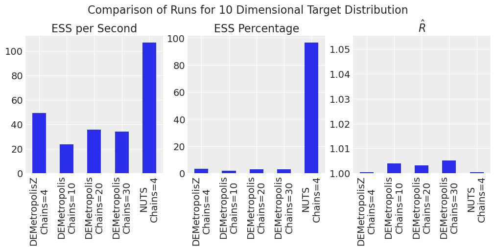
NUTs is the most efficient. DEMetropolisZ is more efficient and has lower \(\hat{R}\) than DEMetropolis.

plot_forest_compare_analytical(results_df)

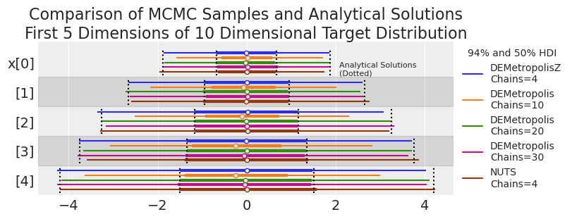
Based on the visual check, the traces have reasonably converged on the target distribution, with the exception of DEMetropolis at 10 chains, supporting the suggestion that the number of chains should be at least 2 times the number of dimensions for a 10 dimensional problem.

Experiment #2. 50-Dimensional Target Distribution

Let’s repeat in 50-dimensions but with even more chains for the DEMetropolis algorithm.

# dimensions
D = 50
# total samples are constant for Metropolis algorithms
total_samples = 200000
samplers = [pm.DEMetropolisZ] + [pm.DEMetropolis] * 3 + [pm.NUTS]
coreses = [1] * 5
chainses = [4, 2 * D, 10 * D, 20 * D, 4]
# calculate the number of tunes and draws for each run
tunes = drawses = [int(total_samples / chains) for chains in chainses]
# manually adjust NUTs, which needs fewer samples
tunes[-1] = drawses[-1] = 2000
# put it in a dataframe for display and QA/QC
pd.DataFrame(
    dict(
        sampler=[s.name for s in samplers],
        tune=tunes,
        draws=drawses,
        chains=chainses,
        cores=coreses,
    )
).style.set_caption("MCMC Runs for 50-Dimensional Experiment")

MCMC Runs for 50-Dimensional Experiment

	sampler	tune	draws	chains	cores
0	DEMetropolisZ	50000	50000	4	1
1	DEMetropolis	2000	2000	100	1
2	DEMetropolis	400	400	500	1
3	DEMetropolis	200	200	1000	1
4	nuts	2000	2000	4	1

results = []
run = 0
for sampler, tune, draws, cores, chains in zip(samplers, tunes, drawses, coreses, chainses):
    if sampler.name == "nuts":
        results.append(
            sample_model_calc_metrics(
                sampler,
                D,
                tune,
                draws,
                cores=cores,
                chains=chains,
                run=run,
                step_kwargs={},
                sample_kwargs=dict(nuts=dict(target_accept=0.95)),
            )
        )
    else:
        results.append(
            sample_model_calc_metrics(sampler, D, tune, draws, cores=cores, chains=chains, run=run)
        )
    run += 1

Show code cell output

Hide code cell output

Sequential sampling (4 chains in 1 job)
DEMetropolisZ: [x]
Sampling 4 chains for 50_000 tune and 50_000 draw iterations (200_000 + 200_000 draws total) took 148 seconds.
The rhat statistic is larger than 1.01 for some parameters. This indicates problems during sampling. See https://arxiv.org/abs/1903.08008 for details
Population sampling (100 chains)
DEMetropolis: [x]
Chains are not parallelized. You can enable this by passing `pm.sample(cores=n)`, where n > 1.
Sampling 100 chains for 2_000 tune and 2_000 draw iterations (200_000 + 200_000 draws total) took 185 seconds.
The rhat statistic is larger than 1.01 for some parameters. This indicates problems during sampling. See https://arxiv.org/abs/1903.08008 for details
The effective sample size per chain is smaller than 100 for some parameters.  A higher number is needed for reliable rhat and ess computation. See https://arxiv.org/abs/1903.08008 for details
Only 400 samples in chain.
Population sampling (500 chains)
DEMetropolis: [x]
Chains are not parallelized. You can enable this by passing `pm.sample(cores=n)`, where n > 1.
Sampling 500 chains for 400 tune and 400 draw iterations (200_000 + 200_000 draws total) took 214 seconds.
c:\Users\greg\.conda\envs\pymc-dev\Lib\site-packages\arviz\data\base.py:221: UserWarning: More chains (500) than draws (400). Passed array should have shape (chains, draws, *shape)
  warnings.warn(
The rhat statistic is larger than 1.01 for some parameters. This indicates problems during sampling. See https://arxiv.org/abs/1903.08008 for details
The effective sample size per chain is smaller than 100 for some parameters.  A higher number is needed for reliable rhat and ess computation. See https://arxiv.org/abs/1903.08008 for details
Only 200 samples in chain.
Population sampling (1000 chains)
DEMetropolis: [x]
Chains are not parallelized. You can enable this by passing `pm.sample(cores=n)`, where n > 1.
Sampling 1000 chains for 200 tune and 200 draw iterations (200_000 + 200_000 draws total) took 245 seconds.
c:\Users\greg\.conda\envs\pymc-dev\Lib\site-packages\arviz\data\base.py:221: UserWarning: More chains (1000) than draws (200). Passed array should have shape (chains, draws, *shape)
  warnings.warn(
The rhat statistic is larger than 1.01 for some parameters. This indicates problems during sampling. See https://arxiv.org/abs/1903.08008 for details
The effective sample size per chain is smaller than 100 for some parameters.  A higher number is needed for reliable rhat and ess computation. See https://arxiv.org/abs/1903.08008 for details
Auto-assigning NUTS sampler...
Initializing NUTS using jitter+adapt_diag...
Sequential sampling (4 chains in 1 job)
NUTS: [x]
Sampling 4 chains for 2_000 tune and 2_000 draw iterations (8_000 + 8_000 draws total) took 94 seconds.
Chain <xarray.DataArray 'chain' ()>
array(0)
Coordinates:
    chain    int32 0 reached the maximum tree depth. Increase `max_treedepth`, increase `target_accept` or reparameterize.
Chain <xarray.DataArray 'chain' ()>
array(1)
Coordinates:
    chain    int32 1 reached the maximum tree depth. Increase `max_treedepth`, increase `target_accept` or reparameterize.
Chain <xarray.DataArray 'chain' ()>
array(2)
Coordinates:
    chain    int32 2 reached the maximum tree depth. Increase `max_treedepth`, increase `target_accept` or reparameterize.
Chain <xarray.DataArray 'chain' ()>
array(3)
Coordinates:
    chain    int32 3 reached the maximum tree depth. Increase `max_treedepth`, increase `target_accept` or reparameterize.

results_df = concat_results(results)
results_df = results_df.reset_index(drop=True)
cols = results_df.columns
results_df[cols[~cols.isin(["Trace", "Run"])]].round(2).style.set_caption(
    "Results of MCMC Sampling of 50-Dimensional Target Distribution"
)

Results of MCMC Sampling of 50-Dimensional Target Distribution

	Sampler	D	Chains	Cores	tune	draws	ESS	Time_sec	ESSperSec	rhat	ESS_pct
0	DEMetropolisZ	50	4	1	50000	50000	1309.830000	163.870000	7.990000	1.000000	0.650000
1	DEMetropolis	50	100	1	2000	2000	792.730000	236.830000	3.350000	1.090000	0.400000
2	DEMetropolis	50	500	1	400	400	1083.880000	415.260000	2.610000	1.410000	0.540000
3	DEMetropolis	50	1000	1	200	200	1616.890000	633.760000	2.550000	1.710000	0.810000
4	NUTS	50	4	1	2000	2000	10570.020000	105.300000	100.380000	1.000000	132.130000

plot_comparison_bars(results_df)

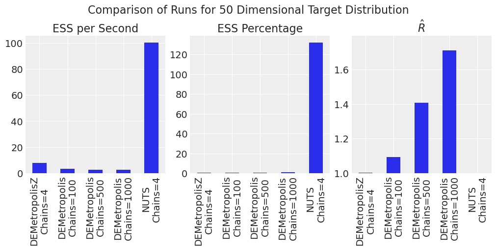
The efficiency advantage for NUTS over DEMetropolisZ over DEMetropolis is more pronounced in higher dimensions. \(\hat{R}\) is also large for DEMetropolis for this sample size and number of chains. For DEMetropolis, a smaller number of chains (\(2N\)) with a larger number of samples performed better than more chains with fewer samples. Counter-intuitively, the NUTS sampler yields \(ESS\) values greater than the number of samples, which can occur as discussed here.

plot_forest_compare_analytical(results_df)

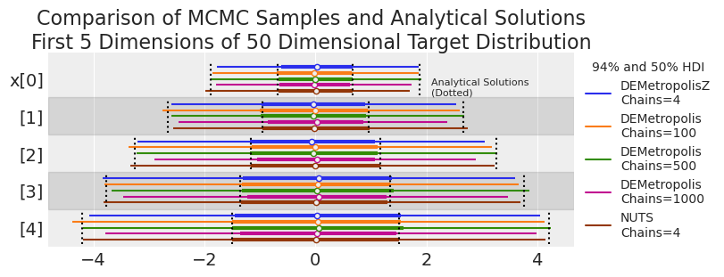
We might be seeing low coverage in the tails of some DEMetropolis runs (i.e., the MCMC HDIs are consistently smaller than the analytical solution). Let’s explore this more systematically in the next experiment.

Experiment #3. Accuracy and Bias

We want to make sure that the DEMetropolis samplers are providing coverage for high dimensional problems (i.e., the tails are appropriately sampled). We will test for bias by running the algorithm multiple times and comparing to both NUTS and the analytically-calculated probability density. We will perform MCMC in many dimensions but analyze the results for the dimension with the most variance (dimension 5) for simplicity.

10 Dimensions

First check in 10 dimensions. We will perform 10 replicates for each run. DEMetropolis will be run at \(2D\) chains. The number of tunes and draws have been tailored to get effective sampler sizes of greater than 2000.

D = 10
reps = 10
samplers = [pm.DEMetropolis] * reps + [pm.DEMetropolisZ] * reps + [pm.NUTS] * reps
coreses = [1] * reps * 3
chainses = [2 * D] * reps + [4] * reps * 2
tunes = drawses = [5000] * reps + [25000] * reps + [1000] * reps

results = []
run = 0
for sampler, tune, draws, cores, chains in zip(samplers, tunes, drawses, coreses, chainses):
    if sampler.name == "nuts":
        results.append(
            sample_model_calc_metrics(
                sampler,
                D,
                tune,
                draws,
                cores=cores,
                chains=chains,
                run=run,
                step_kwargs={},
                sample_kwargs=dict(target_accept=0.95),
            )
        )
    else:
        results.append(
            sample_model_calc_metrics(sampler, D, tune, draws, cores=cores, chains=chains, run=run)
        )
    run += 1

Show code cell output

Hide code cell output

Population sampling (20 chains)
DEMetropolis: [x]
Chains are not parallelized. You can enable this by passing `pm.sample(cores=n)`, where n > 1.
Sampling 20 chains for 5_000 tune and 5_000 draw iterations (100_000 + 100_000 draws total) took 92 seconds.
Population sampling (20 chains)
DEMetropolis: [x]
Chains are not parallelized. You can enable this by passing `pm.sample(cores=n)`, where n > 1.
Sampling 20 chains for 5_000 tune and 5_000 draw iterations (100_000 + 100_000 draws total) took 81 seconds.
Population sampling (20 chains)
DEMetropolis: [x]
Chains are not parallelized. You can enable this by passing `pm.sample(cores=n)`, where n > 1.
Sampling 20 chains for 5_000 tune and 5_000 draw iterations (100_000 + 100_000 draws total) took 81 seconds.
The rhat statistic is larger than 1.01 for some parameters. This indicates problems during sampling. See https://arxiv.org/abs/1903.08008 for details
Population sampling (20 chains)
DEMetropolis: [x]
Chains are not parallelized. You can enable this by passing `pm.sample(cores=n)`, where n > 1.
Sampling 20 chains for 5_000 tune and 5_000 draw iterations (100_000 + 100_000 draws total) took 82 seconds.
The rhat statistic is larger than 1.01 for some parameters. This indicates problems during sampling. See https://arxiv.org/abs/1903.08008 for details
Population sampling (20 chains)
DEMetropolis: [x]
Chains are not parallelized. You can enable this by passing `pm.sample(cores=n)`, where n > 1.
Sampling 20 chains for 5_000 tune and 5_000 draw iterations (100_000 + 100_000 draws total) took 81 seconds.
Population sampling (20 chains)
DEMetropolis: [x]
Chains are not parallelized. You can enable this by passing `pm.sample(cores=n)`, where n > 1.
Sampling 20 chains for 5_000 tune and 5_000 draw iterations (100_000 + 100_000 draws total) took 86 seconds.
The rhat statistic is larger than 1.01 for some parameters. This indicates problems during sampling. See https://arxiv.org/abs/1903.08008 for details
Population sampling (20 chains)
DEMetropolis: [x]
Chains are not parallelized. You can enable this by passing `pm.sample(cores=n)`, where n > 1.
Sampling 20 chains for 5_000 tune and 5_000 draw iterations (100_000 + 100_000 draws total) took 81 seconds.
Population sampling (20 chains)
DEMetropolis: [x]
Chains are not parallelized. You can enable this by passing `pm.sample(cores=n)`, where n > 1.
Sampling 20 chains for 5_000 tune and 5_000 draw iterations (100_000 + 100_000 draws total) took 85 seconds.
The rhat statistic is larger than 1.01 for some parameters. This indicates problems during sampling. See https://arxiv.org/abs/1903.08008 for details
Population sampling (20 chains)
DEMetropolis: [x]
Chains are not parallelized. You can enable this by passing `pm.sample(cores=n)`, where n > 1.
Sampling 20 chains for 5_000 tune and 5_000 draw iterations (100_000 + 100_000 draws total) took 96 seconds.
The rhat statistic is larger than 1.01 for some parameters. This indicates problems during sampling. See https://arxiv.org/abs/1903.08008 for details
Population sampling (20 chains)
DEMetropolis: [x]
Chains are not parallelized. You can enable this by passing `pm.sample(cores=n)`, where n > 1.
Sampling 20 chains for 5_000 tune and 5_000 draw iterations (100_000 + 100_000 draws total) took 86 seconds.
The rhat statistic is larger than 1.01 for some parameters. This indicates problems during sampling. See https://arxiv.org/abs/1903.08008 for details
Sequential sampling (4 chains in 1 job)
DEMetropolisZ: [x]
Sampling 4 chains for 25_000 tune and 25_000 draw iterations (100_000 + 100_000 draws total) took 70 seconds.
Sequential sampling (4 chains in 1 job)
DEMetropolisZ: [x]
Sampling 4 chains for 25_000 tune and 25_000 draw iterations (100_000 + 100_000 draws total) took 77 seconds.
Sequential sampling (4 chains in 1 job)
DEMetropolisZ: [x]
Sampling 4 chains for 25_000 tune and 25_000 draw iterations (100_000 + 100_000 draws total) took 76 seconds.
Sequential sampling (4 chains in 1 job)
DEMetropolisZ: [x]
Sampling 4 chains for 25_000 tune and 25_000 draw iterations (100_000 + 100_000 draws total) took 76 seconds.
Sequential sampling (4 chains in 1 job)
DEMetropolisZ: [x]
Sampling 4 chains for 25_000 tune and 25_000 draw iterations (100_000 + 100_000 draws total) took 79 seconds.
Sequential sampling (4 chains in 1 job)
DEMetropolisZ: [x]
Sampling 4 chains for 25_000 tune and 25_000 draw iterations (100_000 + 100_000 draws total) took 72 seconds.
Sequential sampling (4 chains in 1 job)
DEMetropolisZ: [x]
Sampling 4 chains for 25_000 tune and 25_000 draw iterations (100_000 + 100_000 draws total) took 69 seconds.
Sequential sampling (4 chains in 1 job)
DEMetropolisZ: [x]
Sampling 4 chains for 25_000 tune and 25_000 draw iterations (100_000 + 100_000 draws total) took 77 seconds.
Sequential sampling (4 chains in 1 job)
DEMetropolisZ: [x]
Sampling 4 chains for 25_000 tune and 25_000 draw iterations (100_000 + 100_000 draws total) took 72 seconds.
Sequential sampling (4 chains in 1 job)
DEMetropolisZ: [x]
Sampling 4 chains for 25_000 tune and 25_000 draw iterations (100_000 + 100_000 draws total) took 78 seconds.
Auto-assigning NUTS sampler...
Initializing NUTS using jitter+adapt_diag...
Sequential sampling (4 chains in 1 job)
NUTS: [x]
Sampling 4 chains for 1_000 tune and 1_000 draw iterations (4_000 + 4_000 draws total) took 42 seconds.
Chain <xarray.DataArray 'chain' ()>
array(0)
Coordinates:
    chain    int32 0 reached the maximum tree depth. Increase `max_treedepth`, increase `target_accept` or reparameterize.
Chain <xarray.DataArray 'chain' ()>
array(1)
Coordinates:
    chain    int32 1 reached the maximum tree depth. Increase `max_treedepth`, increase `target_accept` or reparameterize.
Chain <xarray.DataArray 'chain' ()>
array(2)
Coordinates:
    chain    int32 2 reached the maximum tree depth. Increase `max_treedepth`, increase `target_accept` or reparameterize.
Chain <xarray.DataArray 'chain' ()>
array(3)
Coordinates:
    chain    int32 3 reached the maximum tree depth. Increase `max_treedepth`, increase `target_accept` or reparameterize.
Auto-assigning NUTS sampler...
Initializing NUTS using jitter+adapt_diag...
Sequential sampling (4 chains in 1 job)
NUTS: [x]
Sampling 4 chains for 1_000 tune and 1_000 draw iterations (4_000 + 4_000 draws total) took 43 seconds.
Chain <xarray.DataArray 'chain' ()>
array(0)
Coordinates:
    chain    int32 0 reached the maximum tree depth. Increase `max_treedepth`, increase `target_accept` or reparameterize.
Chain <xarray.DataArray 'chain' ()>
array(1)
Coordinates:
    chain    int32 1 reached the maximum tree depth. Increase `max_treedepth`, increase `target_accept` or reparameterize.
Chain <xarray.DataArray 'chain' ()>
array(2)
Coordinates:
    chain    int32 2 reached the maximum tree depth. Increase `max_treedepth`, increase `target_accept` or reparameterize.
Chain <xarray.DataArray 'chain' ()>
array(3)
Coordinates:
    chain    int32 3 reached the maximum tree depth. Increase `max_treedepth`, increase `target_accept` or reparameterize.
Auto-assigning NUTS sampler...
Initializing NUTS using jitter+adapt_diag...
Sequential sampling (4 chains in 1 job)
NUTS: [x]
Sampling 4 chains for 1_000 tune and 1_000 draw iterations (4_000 + 4_000 draws total) took 40 seconds.
Chain <xarray.DataArray 'chain' ()>
array(0)
Coordinates:
    chain    int32 0 reached the maximum tree depth. Increase `max_treedepth`, increase `target_accept` or reparameterize.
Chain <xarray.DataArray 'chain' ()>
array(1)
Coordinates:
    chain    int32 1 reached the maximum tree depth. Increase `max_treedepth`, increase `target_accept` or reparameterize.
Chain <xarray.DataArray 'chain' ()>
array(2)
Coordinates:
    chain    int32 2 reached the maximum tree depth. Increase `max_treedepth`, increase `target_accept` or reparameterize.
Chain <xarray.DataArray 'chain' ()>
array(3)
Coordinates:
    chain    int32 3 reached the maximum tree depth. Increase `max_treedepth`, increase `target_accept` or reparameterize.
Auto-assigning NUTS sampler...
Initializing NUTS using jitter+adapt_diag...
Sequential sampling (4 chains in 1 job)
NUTS: [x]
Sampling 4 chains for 1_000 tune and 1_000 draw iterations (4_000 + 4_000 draws total) took 43 seconds.
Chain <xarray.DataArray 'chain' ()>
array(0)
Coordinates:
    chain    int32 0 reached the maximum tree depth. Increase `max_treedepth`, increase `target_accept` or reparameterize.
Chain <xarray.DataArray 'chain' ()>
array(1)
Coordinates:
    chain    int32 1 reached the maximum tree depth. Increase `max_treedepth`, increase `target_accept` or reparameterize.
Chain <xarray.DataArray 'chain' ()>
array(2)
Coordinates:
    chain    int32 2 reached the maximum tree depth. Increase `max_treedepth`, increase `target_accept` or reparameterize.
Chain <xarray.DataArray 'chain' ()>
array(3)
Coordinates:
    chain    int32 3 reached the maximum tree depth. Increase `max_treedepth`, increase `target_accept` or reparameterize.
Auto-assigning NUTS sampler...
Initializing NUTS using jitter+adapt_diag...
Sequential sampling (4 chains in 1 job)
NUTS: [x]
Sampling 4 chains for 1_000 tune and 1_000 draw iterations (4_000 + 4_000 draws total) took 47 seconds.
Chain <xarray.DataArray 'chain' ()>
array(0)
Coordinates:
    chain    int32 0 reached the maximum tree depth. Increase `max_treedepth`, increase `target_accept` or reparameterize.
Chain <xarray.DataArray 'chain' ()>
array(1)
Coordinates:
    chain    int32 1 reached the maximum tree depth. Increase `max_treedepth`, increase `target_accept` or reparameterize.
Chain <xarray.DataArray 'chain' ()>
array(2)
Coordinates:
    chain    int32 2 reached the maximum tree depth. Increase `max_treedepth`, increase `target_accept` or reparameterize.
Chain <xarray.DataArray 'chain' ()>
array(3)
Coordinates:
    chain    int32 3 reached the maximum tree depth. Increase `max_treedepth`, increase `target_accept` or reparameterize.
Auto-assigning NUTS sampler...
Initializing NUTS using jitter+adapt_diag...
Sequential sampling (4 chains in 1 job)
NUTS: [x]
Sampling 4 chains for 1_000 tune and 1_000 draw iterations (4_000 + 4_000 draws total) took 37 seconds.
Chain <xarray.DataArray 'chain' ()>
array(0)
Coordinates:
    chain    int32 0 reached the maximum tree depth. Increase `max_treedepth`, increase `target_accept` or reparameterize.
Chain <xarray.DataArray 'chain' ()>
array(1)
Coordinates:
    chain    int32 1 reached the maximum tree depth. Increase `max_treedepth`, increase `target_accept` or reparameterize.
Chain <xarray.DataArray 'chain' ()>
array(2)
Coordinates:
    chain    int32 2 reached the maximum tree depth. Increase `max_treedepth`, increase `target_accept` or reparameterize.
Chain <xarray.DataArray 'chain' ()>
array(3)
Coordinates:
    chain    int32 3 reached the maximum tree depth. Increase `max_treedepth`, increase `target_accept` or reparameterize.
Auto-assigning NUTS sampler...
Initializing NUTS using jitter+adapt_diag...
Sequential sampling (4 chains in 1 job)
NUTS: [x]
Sampling 4 chains for 1_000 tune and 1_000 draw iterations (4_000 + 4_000 draws total) took 44 seconds.
Chain <xarray.DataArray 'chain' ()>
array(0)
Coordinates:
    chain    int32 0 reached the maximum tree depth. Increase `max_treedepth`, increase `target_accept` or reparameterize.
Chain <xarray.DataArray 'chain' ()>
array(1)
Coordinates:
    chain    int32 1 reached the maximum tree depth. Increase `max_treedepth`, increase `target_accept` or reparameterize.
Chain <xarray.DataArray 'chain' ()>
array(2)
Coordinates:
    chain    int32 2 reached the maximum tree depth. Increase `max_treedepth`, increase `target_accept` or reparameterize.
Chain <xarray.DataArray 'chain' ()>
array(3)
Coordinates:
    chain    int32 3 reached the maximum tree depth. Increase `max_treedepth`, increase `target_accept` or reparameterize.
Auto-assigning NUTS sampler...
Initializing NUTS using jitter+adapt_diag...
Sequential sampling (4 chains in 1 job)
NUTS: [x]
Sampling 4 chains for 1_000 tune and 1_000 draw iterations (4_000 + 4_000 draws total) took 42 seconds.
Chain <xarray.DataArray 'chain' ()>
array(0)
Coordinates:
    chain    int32 0 reached the maximum tree depth. Increase `max_treedepth`, increase `target_accept` or reparameterize.
Chain <xarray.DataArray 'chain' ()>
array(1)
Coordinates:
    chain    int32 1 reached the maximum tree depth. Increase `max_treedepth`, increase `target_accept` or reparameterize.
Chain <xarray.DataArray 'chain' ()>
array(2)
Coordinates:
    chain    int32 2 reached the maximum tree depth. Increase `max_treedepth`, increase `target_accept` or reparameterize.
Chain <xarray.DataArray 'chain' ()>
array(3)
Coordinates:
    chain    int32 3 reached the maximum tree depth. Increase `max_treedepth`, increase `target_accept` or reparameterize.
Auto-assigning NUTS sampler...
Initializing NUTS using jitter+adapt_diag...
Sequential sampling (4 chains in 1 job)
NUTS: [x]
Sampling 4 chains for 1_000 tune and 1_000 draw iterations (4_000 + 4_000 draws total) took 43 seconds.
Chain <xarray.DataArray 'chain' ()>
array(0)
Coordinates:
    chain    int32 0 reached the maximum tree depth. Increase `max_treedepth`, increase `target_accept` or reparameterize.
Chain <xarray.DataArray 'chain' ()>
array(1)
Coordinates:
    chain    int32 1 reached the maximum tree depth. Increase `max_treedepth`, increase `target_accept` or reparameterize.
Chain <xarray.DataArray 'chain' ()>
array(2)
Coordinates:
    chain    int32 2 reached the maximum tree depth. Increase `max_treedepth`, increase `target_accept` or reparameterize.
Chain <xarray.DataArray 'chain' ()>
array(3)
Coordinates:
    chain    int32 3 reached the maximum tree depth. Increase `max_treedepth`, increase `target_accept` or reparameterize.
Auto-assigning NUTS sampler...
Initializing NUTS using jitter+adapt_diag...
Sequential sampling (4 chains in 1 job)
NUTS: [x]
Sampling 4 chains for 1_000 tune and 1_000 draw iterations (4_000 + 4_000 draws total) took 42 seconds.
Chain <xarray.DataArray 'chain' ()>
array(0)
Coordinates:
    chain    int32 0 reached the maximum tree depth. Increase `max_treedepth`, increase `target_accept` or reparameterize.
Chain <xarray.DataArray 'chain' ()>
array(1)
Coordinates:
    chain    int32 1 reached the maximum tree depth. Increase `max_treedepth`, increase `target_accept` or reparameterize.
Chain <xarray.DataArray 'chain' ()>
array(2)
Coordinates:
    chain    int32 2 reached the maximum tree depth. Increase `max_treedepth`, increase `target_accept` or reparameterize.
Chain <xarray.DataArray 'chain' ()>
array(3)
Coordinates:
    chain    int32 3 reached the maximum tree depth. Increase `max_treedepth`, increase `target_accept` or reparameterize.

results_df = concat_results(results)
results_df = results_df.reset_index(drop=True)
summaries, summary_means = plot_forest_compare_analytical_dim5(results_df)
summary_means.style.set_caption(
    "MCMC and Analytical Results for 5th Dimension of 10 Dimensional Target Distribution"
)

MCMC and Analytical Results for 5th Dimension of 10 Dimensional Target Distribution

	mean	sd	hdi_3%	hdi_97%	ess_bulk	ess_tail	r_hat
Sampler
DEMetropolis	-0.021700	2.214500	-4.125400	4.174200	2772.400000	5331.700000	1.010000
DEMetropolisZ	-0.000200	2.226000	-4.188600	4.159800	3089.100000	5587.200000	1.000000
NUTS	0.001400	2.257800	-4.252700	4.196400	2618.100000	2798.000000	1.000000
Analytical	0.000000	2.236068	-4.205582	4.205582	nan	nan	nan

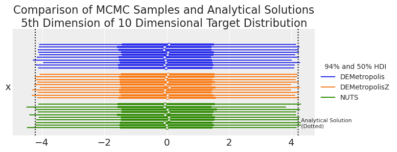
Visually, DEMetropolis algorithms look as reasonable accurate and as accurate as NUTS. Since we have 10 replicates that we want to compare to the analytical solution, we can dust off our traditional statistics and perform an old-school one-sided t-test to see if the sampler-calculated confidence limits are significantly different than the analytically calculated confidence limit.

samplers = ["DEMetropolis", "DEMetropolisZ", "NUTS"]
cls_str = ["hdi_3%", "hdi_97%"]
cls_val = [0.03, 0.97]
dist = st.norm(0, np.sqrt(5))
results = []
for sampler in samplers:
    for cl_str, cl_val in zip(cls_str, cls_val):
        mask = summaries.Sampler == sampler
        # collect the credible limits for each MCMC run
        mcmc_cls = summaries.loc[mask, cl_str]

        # calculate the confidence limit for the target dist
        analytical_cl = dist.ppf(cl_val)

        # one sided t-test!
        p_value = st.ttest_1samp(mcmc_cls, analytical_cl).pvalue
        results.append(
            pd.DataFrame(dict(Sampler=[sampler], ConfidenceLimit=[cl_str], Pvalue=[p_value]))
        )
pd.concat(results).style.set_caption(
    "MCMC Replicates Compared to Analytical Solution for Selected Confidence Limits"
)

MCMC Replicates Compared to Analytical Solution for Selected Confidence Limits

	Sampler	ConfidenceLimit	Pvalue
0	DEMetropolis	hdi_3%	0.018270
0	DEMetropolis	hdi_97%	0.307391
0	DEMetropolisZ	hdi_3%	0.555155
0	DEMetropolisZ	hdi_97%	0.177881
0	NUTS	hdi_3%	0.336053
0	NUTS	hdi_97%	0.847152

A higher p-value indicates that the MCMC algorithm captures the analytical value with high confidence. A lower p-value means that the MCMC algorithm was unexpectedly high or low compared to the analytically calculated confidence limit. The NUTS sampler is capturing the analytically calculated value with high confidence. The DEMetropolis algorithms have lower confidence but are giving reasonable results.

50 Dimensions

Higher dimensions get increasingly difficult for Metropolis algorithms. Here we will sample with very large sample sizes (this will take a while) to get at least 2000 effective samples.

D = 50
reps = 10
samplers = [pm.DEMetropolis] * reps + [pm.DEMetropolisZ] * reps + [pm.NUTS] * reps
coreses = [1] * reps * 3
chainses = [2 * D] * reps + [4] * reps * 2
tunes = drawses = [5000] * reps + [100000] * reps + [1000] * reps

results = []
run = 0
for sampler, tune, draws, cores, chains in zip(samplers, tunes, drawses, coreses, chainses):
    if sampler.name == "nuts":
        results.append(
            sample_model_calc_metrics(
                sampler,
                D,
                tune,
                draws,
                cores=cores,
                chains=chains,
                run=run,
                step_kwargs={},
                sample_kwargs=dict(target_accept=0.95),
            )
        )
    else:
        results.append(
            sample_model_calc_metrics(sampler, D, tune, draws, cores=cores, chains=chains, run=run)
        )
    run += 1

results_df = concat_results(results)
results_df = results_df.reset_index(drop=True)

Show code cell output

Hide code cell output

Population sampling (100 chains)
DEMetropolis: [x]
Chains are not parallelized. You can enable this by passing `pm.sample(cores=n)`, where n > 1.
Sampling 100 chains for 5_000 tune and 5_000 draw iterations (500_000 + 500_000 draws total) took 459 seconds.
The rhat statistic is larger than 1.01 for some parameters. This indicates problems during sampling. See https://arxiv.org/abs/1903.08008 for details
The effective sample size per chain is smaller than 100 for some parameters.  A higher number is needed for reliable rhat and ess computation. See https://arxiv.org/abs/1903.08008 for details
Population sampling (100 chains)
DEMetropolis: [x]
Chains are not parallelized. You can enable this by passing `pm.sample(cores=n)`, where n > 1.
Sampling 100 chains for 5_000 tune and 5_000 draw iterations (500_000 + 500_000 draws total) took 471 seconds.
The rhat statistic is larger than 1.01 for some parameters. This indicates problems during sampling. See https://arxiv.org/abs/1903.08008 for details
The effective sample size per chain is smaller than 100 for some parameters.  A higher number is needed for reliable rhat and ess computation. See https://arxiv.org/abs/1903.08008 for details
Population sampling (100 chains)
DEMetropolis: [x]
Chains are not parallelized. You can enable this by passing `pm.sample(cores=n)`, where n > 1.
Sampling 100 chains for 5_000 tune and 5_000 draw iterations (500_000 + 500_000 draws total) took 473 seconds.
The rhat statistic is larger than 1.01 for some parameters. This indicates problems during sampling. See https://arxiv.org/abs/1903.08008 for details
The effective sample size per chain is smaller than 100 for some parameters.  A higher number is needed for reliable rhat and ess computation. See https://arxiv.org/abs/1903.08008 for details
Population sampling (100 chains)
DEMetropolis: [x]
Chains are not parallelized. You can enable this by passing `pm.sample(cores=n)`, where n > 1.
Sampling 100 chains for 5_000 tune and 5_000 draw iterations (500_000 + 500_000 draws total) took 467 seconds.
The rhat statistic is larger than 1.01 for some parameters. This indicates problems during sampling. See https://arxiv.org/abs/1903.08008 for details
The effective sample size per chain is smaller than 100 for some parameters.  A higher number is needed for reliable rhat and ess computation. See https://arxiv.org/abs/1903.08008 for details
Population sampling (100 chains)
DEMetropolis: [x]
Chains are not parallelized. You can enable this by passing `pm.sample(cores=n)`, where n > 1.
Sampling 100 chains for 5_000 tune and 5_000 draw iterations (500_000 + 500_000 draws total) took 480 seconds.
The rhat statistic is larger than 1.01 for some parameters. This indicates problems during sampling. See https://arxiv.org/abs/1903.08008 for details
The effective sample size per chain is smaller than 100 for some parameters.  A higher number is needed for reliable rhat and ess computation. See https://arxiv.org/abs/1903.08008 for details
Population sampling (100 chains)
DEMetropolis: [x]
Chains are not parallelized. You can enable this by passing `pm.sample(cores=n)`, where n > 1.
Sampling 100 chains for 5_000 tune and 5_000 draw iterations (500_000 + 500_000 draws total) took 466 seconds.
The rhat statistic is larger than 1.01 for some parameters. This indicates problems during sampling. See https://arxiv.org/abs/1903.08008 for details
The effective sample size per chain is smaller than 100 for some parameters.  A higher number is needed for reliable rhat and ess computation. See https://arxiv.org/abs/1903.08008 for details
Population sampling (100 chains)
DEMetropolis: [x]
Chains are not parallelized. You can enable this by passing `pm.sample(cores=n)`, where n > 1.
Sampling 100 chains for 5_000 tune and 5_000 draw iterations (500_000 + 500_000 draws total) took 580 seconds.
The rhat statistic is larger than 1.01 for some parameters. This indicates problems during sampling. See https://arxiv.org/abs/1903.08008 for details
The effective sample size per chain is smaller than 100 for some parameters.  A higher number is needed for reliable rhat and ess computation. See https://arxiv.org/abs/1903.08008 for details
Population sampling (100 chains)
DEMetropolis: [x]
Chains are not parallelized. You can enable this by passing `pm.sample(cores=n)`, where n > 1.
Sampling 100 chains for 5_000 tune and 5_000 draw iterations (500_000 + 500_000 draws total) took 864 seconds.
The rhat statistic is larger than 1.01 for some parameters. This indicates problems during sampling. See https://arxiv.org/abs/1903.08008 for details
The effective sample size per chain is smaller than 100 for some parameters.  A higher number is needed for reliable rhat and ess computation. See https://arxiv.org/abs/1903.08008 for details
Population sampling (100 chains)
DEMetropolis: [x]
Chains are not parallelized. You can enable this by passing `pm.sample(cores=n)`, where n > 1.
Sampling 100 chains for 5_000 tune and 5_000 draw iterations (500_000 + 500_000 draws total) took 878 seconds.
The rhat statistic is larger than 1.01 for some parameters. This indicates problems during sampling. See https://arxiv.org/abs/1903.08008 for details
The effective sample size per chain is smaller than 100 for some parameters.  A higher number is needed for reliable rhat and ess computation. See https://arxiv.org/abs/1903.08008 for details
Population sampling (100 chains)
DEMetropolis: [x]
Chains are not parallelized. You can enable this by passing `pm.sample(cores=n)`, where n > 1.
Sampling 100 chains for 5_000 tune and 5_000 draw iterations (500_000 + 500_000 draws total) took 855 seconds.
The rhat statistic is larger than 1.01 for some parameters. This indicates problems during sampling. See https://arxiv.org/abs/1903.08008 for details
The effective sample size per chain is smaller than 100 for some parameters.  A higher number is needed for reliable rhat and ess computation. See https://arxiv.org/abs/1903.08008 for details
Sequential sampling (4 chains in 1 job)
DEMetropolisZ: [x]
Sampling 4 chains for 100_000 tune and 100_000 draw iterations (400_000 + 400_000 draws total) took 592 seconds.
Sequential sampling (4 chains in 1 job)
DEMetropolisZ: [x]
Sampling 4 chains for 100_000 tune and 100_000 draw iterations (400_000 + 400_000 draws total) took 451 seconds.
Sequential sampling (4 chains in 1 job)
DEMetropolisZ: [x]
Sampling 4 chains for 100_000 tune and 100_000 draw iterations (400_000 + 400_000 draws total) took 429 seconds.
Sequential sampling (4 chains in 1 job)
DEMetropolisZ: [x]
Sampling 4 chains for 100_000 tune and 100_000 draw iterations (400_000 + 400_000 draws total) took 420 seconds.
Sequential sampling (4 chains in 1 job)
DEMetropolisZ: [x]
Sampling 4 chains for 100_000 tune and 100_000 draw iterations (400_000 + 400_000 draws total) took 422 seconds.
Sequential sampling (4 chains in 1 job)
DEMetropolisZ: [x]
Sampling 4 chains for 100_000 tune and 100_000 draw iterations (400_000 + 400_000 draws total) took 425 seconds.
Sequential sampling (4 chains in 1 job)
DEMetropolisZ: [x]
Sampling 4 chains for 100_000 tune and 100_000 draw iterations (400_000 + 400_000 draws total) took 364 seconds.
Sequential sampling (4 chains in 1 job)
DEMetropolisZ: [x]
Sampling 4 chains for 100_000 tune and 100_000 draw iterations (400_000 + 400_000 draws total) took 208 seconds.
Sequential sampling (4 chains in 1 job)
DEMetropolisZ: [x]
Sampling 4 chains for 100_000 tune and 100_000 draw iterations (400_000 + 400_000 draws total) took 206 seconds.
Sequential sampling (4 chains in 1 job)
DEMetropolisZ: [x]
Sampling 4 chains for 100_000 tune and 100_000 draw iterations (400_000 + 400_000 draws total) took 212 seconds.
Auto-assigning NUTS sampler...
Initializing NUTS using jitter+adapt_diag...
Sequential sampling (4 chains in 1 job)
NUTS: [x]
Sampling 4 chains for 1_000 tune and 1_000 draw iterations (4_000 + 4_000 draws total) took 32 seconds.
Chain <xarray.DataArray 'chain' ()>
array(0)
Coordinates:
    chain    int32 0 reached the maximum tree depth. Increase `max_treedepth`, increase `target_accept` or reparameterize.
Chain <xarray.DataArray 'chain' ()>
array(1)
Coordinates:
    chain    int32 1 reached the maximum tree depth. Increase `max_treedepth`, increase `target_accept` or reparameterize.
Chain <xarray.DataArray 'chain' ()>
array(2)
Coordinates:
    chain    int32 2 reached the maximum tree depth. Increase `max_treedepth`, increase `target_accept` or reparameterize.
Chain <xarray.DataArray 'chain' ()>
array(3)
Coordinates:
    chain    int32 3 reached the maximum tree depth. Increase `max_treedepth`, increase `target_accept` or reparameterize.
Auto-assigning NUTS sampler...
Initializing NUTS using jitter+adapt_diag...
Sequential sampling (4 chains in 1 job)
NUTS: [x]
Sampling 4 chains for 1_000 tune and 1_000 draw iterations (4_000 + 4_000 draws total) took 31 seconds.
Chain <xarray.DataArray 'chain' ()>
array(0)
Coordinates:
    chain    int32 0 reached the maximum tree depth. Increase `max_treedepth`, increase `target_accept` or reparameterize.
Chain <xarray.DataArray 'chain' ()>
array(1)
Coordinates:
    chain    int32 1 reached the maximum tree depth. Increase `max_treedepth`, increase `target_accept` or reparameterize.
Chain <xarray.DataArray 'chain' ()>
array(2)
Coordinates:
    chain    int32 2 reached the maximum tree depth. Increase `max_treedepth`, increase `target_accept` or reparameterize.
Chain <xarray.DataArray 'chain' ()>
array(3)
Coordinates:
    chain    int32 3 reached the maximum tree depth. Increase `max_treedepth`, increase `target_accept` or reparameterize.
Auto-assigning NUTS sampler...
Initializing NUTS using jitter+adapt_diag...
Sequential sampling (4 chains in 1 job)
NUTS: [x]
Sampling 4 chains for 1_000 tune and 1_000 draw iterations (4_000 + 4_000 draws total) took 31 seconds.
Chain <xarray.DataArray 'chain' ()>
array(0)
Coordinates:
    chain    int32 0 reached the maximum tree depth. Increase `max_treedepth`, increase `target_accept` or reparameterize.
Chain <xarray.DataArray 'chain' ()>
array(1)
Coordinates:
    chain    int32 1 reached the maximum tree depth. Increase `max_treedepth`, increase `target_accept` or reparameterize.
Chain <xarray.DataArray 'chain' ()>
array(2)
Coordinates:
    chain    int32 2 reached the maximum tree depth. Increase `max_treedepth`, increase `target_accept` or reparameterize.
Chain <xarray.DataArray 'chain' ()>
array(3)
Coordinates:
    chain    int32 3 reached the maximum tree depth. Increase `max_treedepth`, increase `target_accept` or reparameterize.
Auto-assigning NUTS sampler...
Initializing NUTS using jitter+adapt_diag...
Sequential sampling (4 chains in 1 job)
NUTS: [x]
Sampling 4 chains for 1_000 tune and 1_000 draw iterations (4_000 + 4_000 draws total) took 29 seconds.
Chain <xarray.DataArray 'chain' ()>
array(0)
Coordinates:
    chain    int32 0 reached the maximum tree depth. Increase `max_treedepth`, increase `target_accept` or reparameterize.
Chain <xarray.DataArray 'chain' ()>
array(1)
Coordinates:
    chain    int32 1 reached the maximum tree depth. Increase `max_treedepth`, increase `target_accept` or reparameterize.
Chain <xarray.DataArray 'chain' ()>
array(2)
Coordinates:
    chain    int32 2 reached the maximum tree depth. Increase `max_treedepth`, increase `target_accept` or reparameterize.
Chain <xarray.DataArray 'chain' ()>
array(3)
Coordinates:
    chain    int32 3 reached the maximum tree depth. Increase `max_treedepth`, increase `target_accept` or reparameterize.
Auto-assigning NUTS sampler...
Initializing NUTS using jitter+adapt_diag...
Sequential sampling (4 chains in 1 job)
NUTS: [x]
Sampling 4 chains for 1_000 tune and 1_000 draw iterations (4_000 + 4_000 draws total) took 32 seconds.
Chain <xarray.DataArray 'chain' ()>
array(0)
Coordinates:
    chain    int32 0 reached the maximum tree depth. Increase `max_treedepth`, increase `target_accept` or reparameterize.
Chain <xarray.DataArray 'chain' ()>
array(1)
Coordinates:
    chain    int32 1 reached the maximum tree depth. Increase `max_treedepth`, increase `target_accept` or reparameterize.
Chain <xarray.DataArray 'chain' ()>
array(2)
Coordinates:
    chain    int32 2 reached the maximum tree depth. Increase `max_treedepth`, increase `target_accept` or reparameterize.
Chain <xarray.DataArray 'chain' ()>
array(3)
Coordinates:
    chain    int32 3 reached the maximum tree depth. Increase `max_treedepth`, increase `target_accept` or reparameterize.
Auto-assigning NUTS sampler...
Initializing NUTS using jitter+adapt_diag...
Sequential sampling (4 chains in 1 job)
NUTS: [x]
Sampling 4 chains for 1_000 tune and 1_000 draw iterations (4_000 + 4_000 draws total) took 29 seconds.
Chain <xarray.DataArray 'chain' ()>
array(0)
Coordinates:
    chain    int32 0 reached the maximum tree depth. Increase `max_treedepth`, increase `target_accept` or reparameterize.
Chain <xarray.DataArray 'chain' ()>
array(1)
Coordinates:
    chain    int32 1 reached the maximum tree depth. Increase `max_treedepth`, increase `target_accept` or reparameterize.
Chain <xarray.DataArray 'chain' ()>
array(2)
Coordinates:
    chain    int32 2 reached the maximum tree depth. Increase `max_treedepth`, increase `target_accept` or reparameterize.
Chain <xarray.DataArray 'chain' ()>
array(3)
Coordinates:
    chain    int32 3 reached the maximum tree depth. Increase `max_treedepth`, increase `target_accept` or reparameterize.
Auto-assigning NUTS sampler...
Initializing NUTS using jitter+adapt_diag...
Sequential sampling (4 chains in 1 job)
NUTS: [x]
Sampling 4 chains for 1_000 tune and 1_000 draw iterations (4_000 + 4_000 draws total) took 31 seconds.
Chain <xarray.DataArray 'chain' ()>
array(0)
Coordinates:
    chain    int32 0 reached the maximum tree depth. Increase `max_treedepth`, increase `target_accept` or reparameterize.
Chain <xarray.DataArray 'chain' ()>
array(1)
Coordinates:
    chain    int32 1 reached the maximum tree depth. Increase `max_treedepth`, increase `target_accept` or reparameterize.
Chain <xarray.DataArray 'chain' ()>
array(2)
Coordinates:
    chain    int32 2 reached the maximum tree depth. Increase `max_treedepth`, increase `target_accept` or reparameterize.
Chain <xarray.DataArray 'chain' ()>
array(3)
Coordinates:
    chain    int32 3 reached the maximum tree depth. Increase `max_treedepth`, increase `target_accept` or reparameterize.
Auto-assigning NUTS sampler...
Initializing NUTS using jitter+adapt_diag...
Sequential sampling (4 chains in 1 job)
NUTS: [x]
Sampling 4 chains for 1_000 tune and 1_000 draw iterations (4_000 + 4_000 draws total) took 29 seconds.
Chain <xarray.DataArray 'chain' ()>
array(0)
Coordinates:
    chain    int32 0 reached the maximum tree depth. Increase `max_treedepth`, increase `target_accept` or reparameterize.
Chain <xarray.DataArray 'chain' ()>
array(1)
Coordinates:
    chain    int32 1 reached the maximum tree depth. Increase `max_treedepth`, increase `target_accept` or reparameterize.
Chain <xarray.DataArray 'chain' ()>
array(2)
Coordinates:
    chain    int32 2 reached the maximum tree depth. Increase `max_treedepth`, increase `target_accept` or reparameterize.
Chain <xarray.DataArray 'chain' ()>
array(3)
Coordinates:
    chain    int32 3 reached the maximum tree depth. Increase `max_treedepth`, increase `target_accept` or reparameterize.
Auto-assigning NUTS sampler...
Initializing NUTS using jitter+adapt_diag...
Sequential sampling (4 chains in 1 job)
NUTS: [x]
Sampling 4 chains for 1_000 tune and 1_000 draw iterations (4_000 + 4_000 draws total) took 30 seconds.
Chain <xarray.DataArray 'chain' ()>
array(0)
Coordinates:
    chain    int32 0 reached the maximum tree depth. Increase `max_treedepth`, increase `target_accept` or reparameterize.
Chain <xarray.DataArray 'chain' ()>
array(1)
Coordinates:
    chain    int32 1 reached the maximum tree depth. Increase `max_treedepth`, increase `target_accept` or reparameterize.
Chain <xarray.DataArray 'chain' ()>
array(2)
Coordinates:
    chain    int32 2 reached the maximum tree depth. Increase `max_treedepth`, increase `target_accept` or reparameterize.
Chain <xarray.DataArray 'chain' ()>
array(3)
Coordinates:
    chain    int32 3 reached the maximum tree depth. Increase `max_treedepth`, increase `target_accept` or reparameterize.
Auto-assigning NUTS sampler...
Initializing NUTS using jitter+adapt_diag...
Sequential sampling (4 chains in 1 job)
NUTS: [x]
Sampling 4 chains for 1_000 tune and 1_000 draw iterations (4_000 + 4_000 draws total) took 30 seconds.
Chain <xarray.DataArray 'chain' ()>
array(0)
Coordinates:
    chain    int32 0 reached the maximum tree depth. Increase `max_treedepth`, increase `target_accept` or reparameterize.
Chain <xarray.DataArray 'chain' ()>
array(1)
Coordinates:
    chain    int32 1 reached the maximum tree depth. Increase `max_treedepth`, increase `target_accept` or reparameterize.
Chain <xarray.DataArray 'chain' ()>
array(2)
Coordinates:
    chain    int32 2 reached the maximum tree depth. Increase `max_treedepth`, increase `target_accept` or reparameterize.
Chain <xarray.DataArray 'chain' ()>
array(3)
Coordinates:
    chain    int32 3 reached the maximum tree depth. Increase `max_treedepth`, increase `target_accept` or reparameterize.

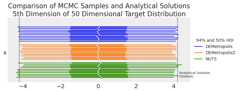
summaries, summary_means = plot_forest_compare_analytical_dim5(results_df)
summary_means.style.set_caption(
    "MCMC and Analytical Results for 5th Dimension of 50 Dimensional Target Distribution"
)

MCMC and Analytical Results for 5th Dimension of 50 Dimensional Target Distribution

	mean	sd	hdi_3%	hdi_97%	ess_bulk	ess_tail	r_hat
Sampler
DEMetropolis	-0.007700	2.236900	-4.224400	4.178500	2583.200000	5619.600000	1.034000
DEMetropolisZ	-0.009700	2.172500	-4.088500	4.079600	2616.800000	5408.700000	1.000000
NUTS	0.030000	2.244200	-4.235000	4.144900	2552.600000	2811.200000	1.000000
Analytical	0.000000	2.236068	-4.205582	4.205582	nan	nan	nan

samplers = ["DEMetropolis", "DEMetropolisZ", "NUTS"]
cls_str = ["hdi_3%", "hdi_97%"]
cls_val = [0.03, 0.97]
results = []
for sampler in samplers:
    for cl_str, cl_val in zip(cls_str, cls_val):
        mask = summaries.Sampler == sampler

        # collect the credible limits for each MCMC run
        mcmc_cls = summaries.loc[mask, cl_str]

        # calculate the confidence limit for the target dist
        analytical_cl = dist.ppf(cl_val)

        # one sided t-test!
        p_value = st.ttest_1samp(mcmc_cls, analytical_cl).pvalue

        results.append(
            pd.DataFrame(dict(Sampler=[sampler], ConfidenceLimit=[cl_str], Pvalue=[p_value]))
        )
pd.concat(results).style.set_caption(
    "MCMC Replicates Compared to Analytical Solution for Selected Confidence Limits"
)

MCMC Replicates Compared to Analytical Solution for Selected Confidence Limits

	Sampler	ConfidenceLimit	Pvalue
0	DEMetropolis	hdi_3%	0.152028
0	DEMetropolis	hdi_97%	0.318463
0	DEMetropolisZ	hdi_3%	0.001217
0	DEMetropolisZ	hdi_97%	0.005154
0	NUTS	hdi_3%	0.490542
0	NUTS	hdi_97%	0.212516

We can see that at 50 dimensions, the DEMetropolisZ sampler has poor coverage compared to DEMetropolis. Therefore, even though DEMetropolisZ is more efficient and has lower \(\hat{R}\) values than DEMetropolis, DEMetropolis is suggested for higher dimensional problems.

Conclusion

Based on the results in this notebook, if you cannot use NUTS, use DEMetropolisZ for lower dimensional problems (e.g., \(10D\)) because it is more efficient and converges better. Use DEMetropolis for higher dimensional problems (e.g., \(50D\)) to better capture the tails of the target distribution.

%load_ext watermark
%watermark -n -u -v -iv -w

Last updated: Fri Feb 10 2023

Python implementation: CPython
Python version       : 3.11.0
IPython version      : 8.7.0

pymc      : 5.0.1+5.ga7f361bd
numpy     : 1.24.0
pandas    : 1.5.2
sys       : 3.11.0 | packaged by conda-forge | (main, Oct 25 2022, 06:12:32) [MSC v.1929 64 bit (AMD64)]
matplotlib: 3.6.2
scipy     : 1.9.3
arviz     : 0.14.0

Watermark: 2.3.1